library(rstanarm)
library(shinystan)

df <- read.csv(url("https://raw.githubusercontent.com/NERC-CEH/beem_data/main/trees.csv"))
df$basal_area <- pi * (df$dbh/2)^2Model Selection and Comparison
Introduction
In this practical, we are going to go back over the models fit within the linear modelling practical session 3a and assess their fit in more detail and compare different models.
Tree allometry models
Model evaluation
Yesterday, we were looking at fitting different models to tree mass data. In the practical session there were multiple variables to include within the tree mass model and the code below was included to show the full list of potential metrics.
Remember to load the libraries and read in the data exactly as in the previous practical session
Now we can fit the linear model with multiple predictor variables
m_multi <- stan_glm(tree_mass ~ basal_area +
  age + species + cultivation + soil_type + tree_height + timber_height,
  data = df, refresh = 0)

summary(m_multi)
Model Info:
 function:     stan_glm
 family:       gaussian [identity]
 formula:      tree_mass ~ basal_area + age + species + cultivation + soil_type +
       tree_height + timber_height
 algorithm:    sampling
 sample:       4000 (posterior sample size)
 priors:       see help('prior_summary')
 observations: 1881
 predictors:   34

Estimates:
                mean   sd     10%    50%    90%
(Intercept)   -202.8   13.8 -220.5 -202.6 -184.8
basal_area       0.8    0.0    0.8    0.8    0.8
age             -0.3    0.4   -0.7   -0.3    0.2
speciesDF       23.4   14.9    4.0   23.6   42.6
speciesEL        0.1   16.1  -20.0   -0.2   21.4
speciesGF      -17.0   14.3  -35.3  -16.9    1.4
speciesJL      -14.8   12.9  -31.3  -14.8    2.0
speciesLC       51.1   28.3   14.9   50.9   87.4
speciesLP       18.9    9.5    6.9   18.6   31.1
speciesNF       43.0   18.7   19.5   42.9   66.8
speciesNS       28.6   10.2   15.6   28.4   41.8
speciesRC      -58.4   25.2  -91.1  -58.1  -25.7
speciesSP        4.9    9.8   -7.6    4.9   17.3
speciesSS       32.2    8.6   21.2   32.2   43.2
speciesWH       13.3   13.3   -3.6   13.4   30.0
cultivation     -0.1    0.7   -1.0   -0.1    0.9
soil_type10     -8.9   17.9  -31.9   -9.3   14.5
soil_type11    -67.5   16.4  -88.7  -67.2  -46.8
soil_type12    -59.1   16.6  -80.6  -59.4  -37.8
soil_type13    -93.3   24.1 -123.3  -93.7  -62.3
soil_type1a     -1.5   23.4  -31.4   -1.4   28.2
soil_type1g     -9.1   14.7  -28.1   -8.9   10.2
soil_type1x    -18.5   17.7  -41.1  -18.5    3.8
soil_type3       0.9    7.3   -8.6    1.0   10.2
soil_type4       3.1    7.7   -6.6    3.0   12.9
soil_type4b     -2.8   10.2  -15.6   -2.7   10.2
soil_type5b    -21.4   11.4  -36.1  -21.3   -6.9
soil_type6     -10.6    6.0  -18.3  -10.7   -2.8
soil_type7       8.9    6.1    1.1    8.9   16.8
soil_type7b   -241.6   13.0 -258.1 -241.5 -224.7
soil_type8       1.1   25.1  -31.4    1.1   33.0
soil_type9      -4.8    8.5  -15.9   -4.8    6.0
tree_height      5.2    2.0    2.5    5.3    7.8
timber_height   13.3    2.1   10.6   13.3   16.2
sigma           65.7    1.1   64.3   65.6   67.1

Fit Diagnostics:
           mean   sd    10%   50%   90%
mean_PPD 325.4    2.1 322.7 325.3 328.2

The mean_ppd is the sample average posterior predictive distribution of the outcome variable (for details see help('summary.stanreg')).

MCMC diagnostics
              mcse Rhat n_eff
(Intercept)   0.3  1.0  1899
basal_area    0.0  1.0  4549
age           0.0  1.0  3376
speciesDF     0.3  1.0  2046
speciesEL     0.4  1.0  2114
speciesGF     0.3  1.0  1920
speciesJL     0.3  1.0  1990
speciesLC     0.4  1.0  4789
speciesLP     0.3  1.0  1283
speciesNF     0.3  1.0  2994
speciesNS     0.3  1.0  1352
speciesRC     0.4  1.0  4849
speciesSP     0.2  1.0  1589
speciesSS     0.3  1.0  1110
speciesWH     0.3  1.0  1976
cultivation   0.0  1.0  5431
soil_type10   0.2  1.0  6150
soil_type11   0.2  1.0  5375
soil_type12   0.3  1.0  4423
soil_type13   0.3  1.0  6711
soil_type1a   0.3  1.0  5880
soil_type1g   0.2  1.0  5727
soil_type1x   0.2  1.0  5318
soil_type3    0.1  1.0  2419
soil_type4    0.2  1.0  1636
soil_type4b   0.2  1.0  2746
soil_type5b   0.2  1.0  2634
soil_type6    0.1  1.0  1860
soil_type7    0.1  1.0  2295
soil_type7b   0.2  1.0  3618
soil_type8    0.3  1.0  6156
soil_type9    0.2  1.0  2747
tree_height   0.0  1.0  1859
timber_height 0.1  1.0  1759
sigma         0.0  1.0  3635
mean_PPD      0.0  1.0  3898
log-posterior 0.1  1.0  1476

For each parameter, mcse is Monte Carlo standard error, n_eff is a crude measure of effective sample size, and Rhat is the potential scale reduction factor on split chains (at convergence Rhat=1).
Your task within this practical is to fit different versions of this model with different terms in (perhaps even polynomial terms) and to evaluate the model fit of each.
To launch shinystan and evaluate the different properties of the model fit, use:
launch_shinystan(m_multi)Take time to understand the different aspects of the model fit, taking particular notice of the effective sample size and the Monte Carlo standard error.
We can also visualise the fit using the posterior check:
pp_check(m_multi)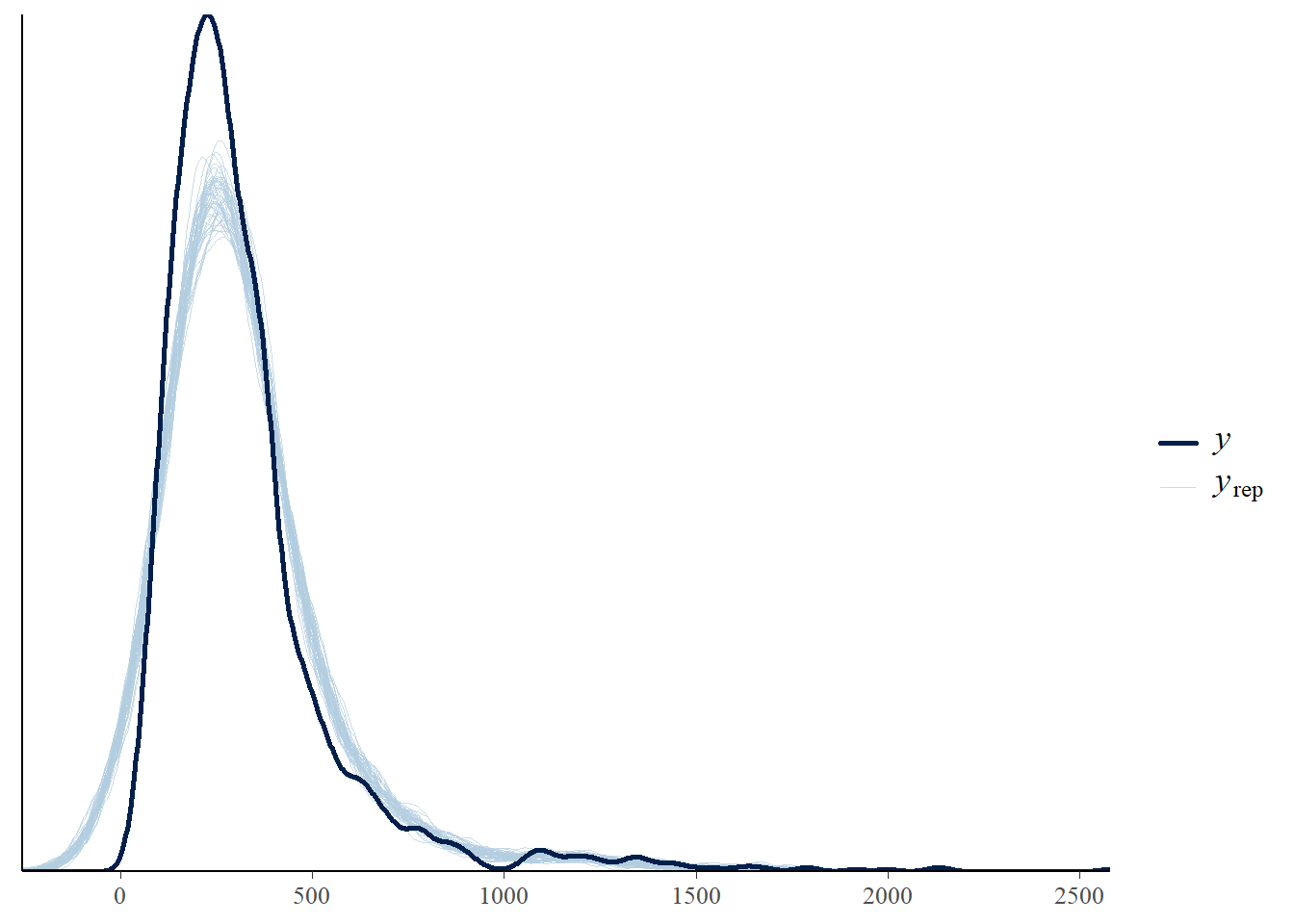
Try this for at least 4 or 5 different versions of the model, noting which you believe to be the most appropriate and why.
Model comparison
Now we will use the loo package to formally compare different models.
So lets fit a second model that includes a polynomial of order 2 (a squared term) for age. Our aim is to adequately evaluate and compare this model with the original to understand if this is a significant improvement
Fit the model using the following code
m_multi_2 <- update(m_multi, formula. = . ~ . + I(age^2))Now run through the checks as above to evaluate this new model. If all seems to be reasonable, we can consider at this stage if we believe one model to be “better” than the other. The posterior predictive check is useful for this.
But we can also compare the models more formally, using both leave one out cross validation and the WAIC.
library(loo)

#run the efficient LOO CV on the 2 different models using the loo package
loo_m_1 <- loo(m_multi)
loo_m_2 <- loo(m_multi_2)
Now we have evaluated the loo cv, we can view the diagnostic for each observation as it was left out. This helps to understand the leverage of different observations - similar to cook’s distance that is often used.
par(mfrow = c(1,2))
plot(loo_m_1, label_points = TRUE)
plot(loo_m_2, label_points = TRUE)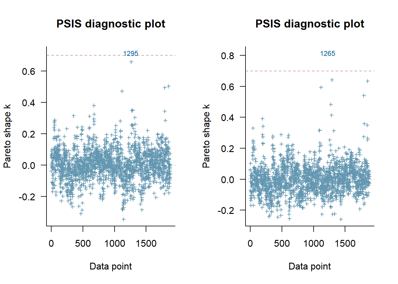
This plot shows only a very outliers for either model, and so nothing to worry about.
Finally, we can directly compare the diagnostics from the 2 models to see which is more appropriate.
loo_compare(loo_m_1, loo_m_2) elpd_diff se_diff
m_multi_2 0.0 0.0
m_multi -86.5 20.6 In this case, there is quite a large difference in the expected log pointwise deviance between the two models compared to the standard error of that difference, so we are led to favour the model with the additional squared term, even after taking into account that the second model estimates an additional parameter.
Try comparing other models in the same way. Do higher polynomials continue to improve the fit?